-
(DACON) 영화 관객수 예측 튜토리얼 대회IT 지식 창고 2019. 7. 7. 16:46
데이콘에서 주최하는 제 1회 튜토리얼 대회
https://dacon.io/tutorial_comp/87871
튜토리얼
dacon.io
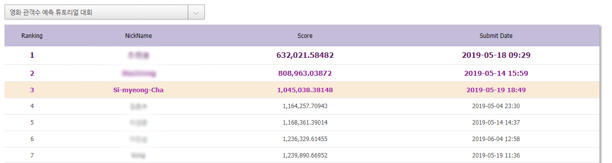
전체 44명 중에서 3등을 하였지만, 외부데이터 사용과정에서 Data leakage issue가 있어 실격처리 되어 수상하지 못하였습니다.
하지만, 외부데이터를 크롤링하는 과정을 공부하게 되었고 외부데이터를 사용하지 않아도 110만점에 가까운 Score를 얻을 수 있던 의미있는 코드라고 생각합니다.
영화 관객수 예측 정리 In [1]:#주피터 노트북 블로그게시용 함수 from IPython.core.display import display, HTML display(HTML("<style> .container{width:100% !important;}</style>"))
In [1]:# For example, here's several helpful packages to load in import numpy as np # linear algebra import pandas as pd # data processing, CSV file I/O (e.g. pd.read_csv) import matplotlib.pyplot as plt #data visualization import seaborn as sns import warnings warnings.filterwarnings("ignore") # Input data files are available in the "../영화관객수예측/" directory. # For example, running this (by clicking run or pressing Shift+Enter) will list the files in the input directory import os print(os.listdir("../영화관객수예측/")) # Any results you write to the current directory are saved as output. import sys print ('Python version ->', sys.version) print ('Numpy version ->', np.__version__) print ('Pandas version ->', pd.__version__)
1. Data set 불러오기
In [2]:train_df = pd.read_csv('../영화관객수예측/movies_train.csv') # training dataframe test_df = pd.read_csv('../영화관객수예측/movies_test.csv')# testing dataframe
In [3]:#원본데이터는 보존하기 위함 train = train_df.copy() test = test_df.copy()
In [4]:print("train.csv. Shape: ",train.shape) print("test.csv. Shape: ",test.shape)
In [5]:train_null = train.drop('box_off_num', axis = 1).isnull().sum()/len(train)*100 test_null = test.isnull().sum()/len(test)*100 pd.DataFrame({'train_null_count' : train_null, 'test_null_count' : test_null})
Out[5]:missing data는 dir_prev_bfnum가 55%정도 있습니다. 그외에는 없습니다.
In [6]:train.info()
NAVER 검색 API사용
naver에서 제공하는 검색 API에서 평점이라는 데이터를 가지고 새로운 피쳐를 생성합니다.
train
In [7]:# import os # import sys # import urllib.request # import json # import time # import timeit # start = timeit.default_timer() # count = 0 # #API 사용 아이디 및 비밀번호 # client_id = "Fo_P8tuHi5_qUQUIGIWp" # client_secret = "nwKNomCW5F" # train_title = train.loc[:,'title'] # train_director = train.loc[:,'director'] # train['user_rating'] = 0 # for movie, name in zip(train_title, train_director): # if count == 30: # count = 0 # title = movie # director = name + '|' # encText = urllib.parse.quote(title) # display = '&display=100' # yearfrom = '&yearfrom=2010' # yearto = '&yearto=2015' # url = "https://openapi.naver.com/v1/search/movie?query=" + encText + display + yearfrom + yearto # json 결과 # # url = "https://openapi.naver.com/v1/search/blog.xml?query=" + encText # xml 결과 # request = urllib.request.Request(url) # request.add_header("X-Naver-Client-Id",client_id) # request.add_header("X-Naver-Client-Secret",client_secret) # response = urllib.request.urlopen(request) # rescode = response.getcode() # if(rescode==200): # response_body = response.read() # else: # print("Error Code:" + rescode) # break # result = json.loads(response_body) # for i in range(len(result['items'])): # if result['items'][i]['director'] == director: # train.loc[train['title']==title, 'user_rating'] = result['items'][i]['userRating'] # count += 1 # if count == 30: # time.sleep(1) # stop = timeit.default_timer() # print('불러오는데 걸린 시간 : {}초'.format(stop - start)) # print('rating이 0인 row 갯수 : {}개'.format(len(train[train['user_rating']==0])))
감독이나, 년도가 달라서 데이터가 0인 경우는 다시 조건을 넓혀 검색해봄
In [8]:# import os # import sys # import urllib.request # import json # start = timeit.default_timer() # count = 0 # client_id = "Fo_P8tuHi5_qUQUIGIWp" # client_secret = "nwKNomCW5F" # train_title = train.loc[train['user_rating']==0,'title'] # train_director = train.loc[train['user_rating']==0,'director'] # for movie, name in zip(train_title, train_director): # if count == 30: # count = 0 # title = movie # director = name + '|' # encText = urllib.parse.quote(title) # display = '&display=100' # url = "https://openapi.naver.com/v1/search/movie?query=" + encText # json 결과 # # url = "https://openapi.naver.com/v1/search/blog.xml?query=" + encText # xml 결과 # request = urllib.request.Request(url) # request.add_header("X-Naver-Client-Id",client_id) # request.add_header("X-Naver-Client-Secret",client_secret) # response = urllib.request.urlopen(request) # rescode = response.getcode() # if(rescode==200): # response_body = response.read() # else: # print("Error Code:" + rescode) # break # result = json.loads(response_body) # for i in range(len(result['items'])): # if result['items'][i]['director'] == director: # train.loc[train['title']==title, 'user_rating'] = result['items'][i]['userRating'] # count += 1 # if count == 30: # time.sleep(1) # stop = timeit.default_timer() # print('불러오는데 걸린 시간 : {}초'.format(stop - start)) # print('rating이 0인 row 갯수 : {}개'.format(len(train[train['user_rating']==0])))
test
In [9]:# start = timeit.default_timer() # count = 0 # client_id = "Fo_P8tuHi5_qUQUIGIWp" # client_secret = "nwKNomCW5F" # test_title = test.loc[:,'title'] # test_director = test.loc[:,'director'] # test['user_rating'] = 0 # for movie, name in zip(test_title, test_director): # if count == 30: # count = 0 # title = movie # director = name + '|' # encText = urllib.parse.quote(title) # display = '&display=100' # yearfrom = '&yearfrom=2010' # yearto = '&yearto=2015' # url = "https://openapi.naver.com/v1/search/movie?query=" + encText + display + yearfrom + yearto # json 결과 # # url = "https://openapi.naver.com/v1/search/blog.xml?query=" + encText # xml 결과 # request = urllib.request.Request(url) # request.add_header("X-Naver-Client-Id",client_id) # request.add_header("X-Naver-Client-Secret",client_secret) # response = urllib.request.urlopen(request) # rescode = response.getcode() # if(rescode==200): # response_body = response.read() # else: # print("Error Code:" + rescode) # break # result = json.loads(response_body) # for i in range(len(result['items'])): # if result['items'][i]['director'] == director: # test.loc[test['title']==title, 'user_rating'] = result['items'][i]['userRating'] # count += 1 # if count == 30: # time.sleep(1) # stop = timeit.default_timer() # print('불러오는데 걸린 시간 : {}초'.format(stop - start)) # print('rating이 0인 row 갯수 : {}개'.format(len(test[test['user_rating']==0])))
In [10]:# start = timeit.default_timer() # count = 0 # client_id = "Fo_P8tuHi5_qUQUIGIWp" # client_secret = "nwKNomCW5F" # test_title = test.loc[test['user_rating']==0,'title'] # test_director = test.loc[test['user_rating']==0,'director'] # for movie, name in zip(test_title, test_director): # if count == 30: # count = 0 # title = movie # director = name + '|' # encText = urllib.parse.quote(title) # display = '&display=100' # url = "https://openapi.naver.com/v1/search/movie?query=" + encText # json 결과 # # url = "https://openapi.naver.com/v1/search/blog.xml?query=" + encText # xml 결과 # request = urllib.request.Request(url) # request.add_header("X-Naver-Client-Id",client_id) # request.add_header("X-Naver-Client-Secret",client_secret) # response = urllib.request.urlopen(request) # rescode = response.getcode() # if(rescode==200): # response_body = response.read() # else: # print("Error Code:" + rescode) # result = json.loads(response_body) # for i in range(len(result['items'])): # if result['items'][i]['director'] == director: # test.loc[test['title']==title, 'user_rating'] = result['items'][i]['userRating'] # count += 1 # if count == 30: # time.sleep(1) # stop = timeit.default_timer() # print('불러오는데 걸린 시간 : {}초'.format(stop - start)) # print('rating이 0인 row 갯수 : {}개'.format(len(test[test['user_rating']==0])))
In [11]:# train[['title', 'user_rating']].to_csv('rate_train.csv', index=False) # test[['title', 'user_rating']].to_csv('rate_test.csv', index=False)
In [12]:#외부데이터(user_rating)이 포함된 csv파일 rate_train = pd.read_csv('../영화관객수예측/rate_train.csv') # user rating train rate_test = pd.read_csv('../영화관객수예측/rate_test.csv')# user rating test
In [13]:train = pd.merge(train, rate_train, on='title') test = pd.merge(test, rate_test, on='title')
2. Exploratory Data Analysis AND Processing
Column_name Description
- title : 영화의 제목
- distributor : 배급사
- genre : 장르
- release_time : 개봉일
- time : 상영시간(분)
- screening_rat : 상영등급
- director : 감독이름
- dir_prev_bfnum : 해당 감독이 이 영화를 만들기 전 제작에 참여한 영화에서의 평균 관객수(단 관객수가 알려지지 않은 영화 제외)
- dir_prev_num : 해당 감독이 이 영화를 만들기 전 제작에 참여한 영화의 개수(단 관객수가 알려지지 않은 영화 제외)
- num_staff : 스텝수
- num_actor : 주연배우수
- box_off_num : 관객수
- user_rating(외부데이터) : 네이버에서 제공하는 평점 데이터
데이터 탐색 과정에서 이상한 값들이 있어서.. 미리 삭제하고 시작하겠습니다.
In [14]:#슈퍼레이서 엔지의 time이 release_time데이터로 있어서 값을 수정하겠습니다. test.loc[test['title'] == '슈퍼레이서 엔지', 'time'] = 63 #시리즈물중에 중복되어있어서 값을 수정하는 것 보다 삭제를 하겠습니다. train.drop([10, 311], inplace=True)
2.1 Target Variable (Dependent Variable)
box_off_num : 관객수
In [15]:train['box_off_num'].describe()
Out[15]:- 총 600개의 데이터
- 평균 : 708181.8 약 70만
- 표준편차 : 1828006 약 180만
- min : 1
- max : 14262770 약 1400만
In [16]:f, ax = plt.subplots(figsize = (8,6)) sns.distplot(train['box_off_num']) print("%s -> Skewness: %f, Kurtosis: %f" % ('box_off_num',train['box_off_num'].skew(), train['box_off_num'].kurt()))

- 왜도(Skewness) : 왼쪽으로 치우쳐져 있을수록 값이크고, 오른쪽으로 치우쳐져 있을 수록 값이 작아진다. 즉, 0에 가까울수록 좋은 형태
- 첨도(Kurtosis) : 첨도 값이 3에 가까울 경우 정규분포에 가까우며, 첨도 값이 클수록 뾰족하고 값이 작을 수록 완만해진다
In [17]:train['box_off_num'] = np.log1p(train['box_off_num']) print("%s -> Skewness: %f, Kurtosis: %f" % ('box_off_num',train['box_off_num'].skew(), train['box_off_num'].kurt()))
In [18]:f, ax = plt.subplots(figsize = (8,6)) sns.distplot(train['box_off_num'])
Out[18]:
2.2 Missing data
missing data가 있는 dir_prev_bfnum 부터 확인하겠습니다.
dir_prev_bfnum
감독이 해당 영화를 만들 기 전의 평균 관객수
In [19]:#Nan값을 제외한 데이터 히스토그램 분포 f, ax = plt.subplots(figsize = (8,6)) train_bfnum = train[train['dir_prev_bfnum'].notnull()] sns.distplot(train_bfnum['dir_prev_bfnum']) print("%s -> Skewness: %f, Kurtosis: %f" % ('dir_prev_bfnum',train_bfnum['dir_prev_bfnum'].skew(), train_bfnum['dir_prev_bfnum'].kurt()))

대부분이 작은 값을 가지고 있습니다.
dir_prev_bfnum은 감독이 해당영화 만들기전의 평균 관객수입니다.
하나의 영화를 만들었다면 과거데이터가 없어서 값이 없을 수도 있습니다.
따라서 1개의 영화를 만든 감독은 0의 데이터를 집어넣겠습니다.
In [20]:#train과 test를 합침 all_data = pd.concat([train, test], sort=False).reset_index(drop=True) print('Null count :',all_data['dir_prev_bfnum'].isnull().sum()) #dir_prev_bfnum에서 NaN값을 가지고 있는 데이터를 따로 만듬 bfnum_null = all_data[all_data['dir_prev_bfnum'].isnull()] #NaN 값중 감독별 영화갯수가 몇개인지 확인 director_count = bfnum_null[['title','director']].groupby('director').count() director_count = director_count.reset_index() print('Director Null count :',director_count['director'].count()) #영화가 1개인 경우는 이전의 영화가 없어서 NaN값일 수 도 있으므로 감독의 이름을 가져오기 위해 #또 새로운 데이터프레임을 만들고 해당하는 감독의 영화는 0으로 채워 넣는다. dire_1 = director_count[director_count['title']==1]['director'] for name in dire_1: all_data.loc[all_data['director']==name, 'dir_prev_bfnum'] = all_data.loc[all_data['director']==name, 'dir_prev_bfnum'].fillna(0)
나머지 null값에 대해서 확인해보겠습니다.
In [21]:print('Null count :',all_data['dir_prev_bfnum'].isnull().sum()) #위와 똑같은 과정 반복 #한 감독이 2개 이상 만든 경우의 NaN 데이터프레임 생성 bfnum_null = all_data[all_data['dir_prev_bfnum'].isnull()] director_count = bfnum_null[['title','director']].groupby('director').count() director_count = director_count.reset_index() print('Director Null count :',director_count['director'].count()) #관람객 수를 log취했기 때문에 원래대로 돌려 bfnum을 채우기 위한 용도로 사용. all_data['box_off_num'] = np.expm1(all_data['box_off_num'])
In [22]:#데이터를 순서대로 평균값을 계산하고 채워 넣을 수 있도록 사용자 정의 함수 만듬 def director_bfnum(all_director): #만약 첫번째 bfnum의 값이 있다면 그대로 두고, 없다면 다 0으로 채워 넣음 if pd.isnull(all_director.iloc[0, 7]): all_director.iloc[0, 7] = 0 count = 1 num = 0 #순차적으로 bfnum과 box_off_num을 더하여 갯수만큼 나눌 수 있는 평균을 구하도록함 for i in range(1, len(all_director)): num += all_director['box_off_num'].iloc[i-1] bfnum = num/count all_director.iloc[i, 7] = bfnum count += 1 return all_director
In [23]:#2개 이상인 데이터의 감독명을 받아옴 dire_2 = director_count['director'] #test데이터도 계산을 위해 nan값을 0의 값으로 가져온다. #train과 test로 나눌 때 삭제해야함 all_data['box_off_num'].fillna(0, inplace=True) for name in dire_2: all_director = all_data[all_data['director'] == name].sort_values('release_time') all_data[all_data['director']==name] = director_bfnum(all_director)
In [24]:#원래의 데이터로 다 돌려줌 ntrain = len(train) train = all_data[:ntrain] test = all_data[ntrain:] test.drop('box_off_num', axis=1, inplace=True) train['box_off_num'] = np.log1p(train['box_off_num'])
In [25]:train_null = train.drop('box_off_num', axis = 1).isnull().sum()/len(train)*100 test_null = test.isnull().sum()/len(test)*100 pd.DataFrame({'train_null_count' : train_null, 'test_null_count' : test_null})
Out[25]:말끔 ㅎㅎ..
겸사겸사 왜도, 첨도도 조사하여 조정해주겠습니다.
In [26]:f, ax = plt.subplots(figsize = (8,6)) sns.distplot(train['dir_prev_bfnum']) print("%s -> Skewness: %f, Kurtosis: %f" % ('dir_prev_bfnum',train_bfnum['dir_prev_bfnum'].skew(), train_bfnum['dir_prev_bfnum'].kurt()))
 In [27]:
train['dir_prev_bfnum'] = np.log1p(train['dir_prev_bfnum'])
test['dir_prev_bfnum'] = np.log1p(test['dir_prev_bfnum'])
print("%s -> Skewness: %f, Kurtosis: %f" %  ('dir_prev_bfnum',train['dir_prev_bfnum'].skew(),
                                                     train['dir_prev_bfnum'].kurt()))
In [28]:f, ax = plt.subplots(figsize = (8,6)) sns.distplot(train['dir_prev_bfnum'])
Out[28]:
dir_prev_num
dir_prev_num이 0인데 dir_prev_bfnum이 값을 가진 경우가 있습니다.
이 경우에 감독이 영화를 하나만 만든경우는 1을 넣어주겠습니다.
In [29]:#train과 test를 합침 all_data = pd.concat([train, test], sort=False).reset_index(drop=True) #num이 0인데 값을 가진 경우를 새로운 데이터프레임으로 만듬 num_group = all_data[(all_data['dir_prev_num']==0) & (all_data['dir_prev_bfnum']>0)].groupby('director')[['dir_prev_num']].count().reset_index() print('num_zero count : ', num_group['dir_prev_num'].count()) #해당하는 감독의 이름을 가져오기 위한 데이터프레임을 새로 생성 dire_1 = num_group[num_group['dir_prev_num']==1]['director'] for name in dire_1: all_data.loc[all_data['director']==name, 'dir_prev_num'] = 1
그 외 데이터에 대해서 첫번째 num 값 이후로 순차적으로 데이터를 넣어주겠습니다.
In [30]:def director_num(prev_num): count = prev_num.iloc[0, 8] for i in range(1, len(prev_num)): prev_num.iloc[i, 8] = count count+=1 return prev_num director = all_data['director'] for name in director: prev_num = all_data[all_data['director'] == name].sort_values('release_time') all_data[all_data['director']==name] = director_num(prev_num)
In [31]:#원래의 데이터로 다 돌려줌 ntrain = len(train) train = all_data[:ntrain] test = all_data[ntrain:] test.drop('box_off_num', axis=1, inplace=True)
In [32]:f, ax = plt.subplots(figsize = (8,6)) sns.boxplot(train['dir_prev_num'], train['box_off_num'])
Out[32]:
columns 상관관계
In [33]:#상관관계 확인 k=20 #히트맵 변수 갯수 corrmat = train.corr() #변수간의 상관관계 cols = corrmat.nlargest(k, 'box_off_num')['box_off_num'].index #price기준으로 제일 큰순서대로 20개를 뽑아냄 cm = np.corrcoef(train[cols].values.T) f, ax = plt.subplots(figsize=(8, 6)) sns.heatmap(data = cm, annot=True, square=True, fmt = '.2f', linewidths=.5, cmap='Reds', yticklabels = cols.values, xticklabels = cols.values)
Out[33]:
2.3 Categorical Variable
distributor (배급사)
object인 데이터들 우선적으로 탐색하며 데이터를 변형하겠습니다.
In [34]:dis_unique = train['distributor'].unique() len(dis_unique)
Out[34]:In [35]:train_dist = train[['box_off_num','distributor']].groupby('distributor').mean().sort_values('box_off_num').reset_index() train_dist.head()
Out[35]:In [36]:dist_num = {} for i in range(len(train_dist)): distributor = train_dist['distributor'].iloc[i] dist_num[distributor] = i
In [37]:train_test_data = [train, test] for dataset in train_test_data: dataset['distributor'] = dataset['distributor'].map(dist_num)
test에는 train의 distributor가 없는 경우도 있기때문에
NaN값은 우선 0으로 채워넣겠습니다.
In [38]:test['distributor'].fillna(0, inplace = True)
screening_rat
In [39]:train['screening_rat'].unique()
Out[39]:In [40]:replace_name = {'청소년 관람불가' : 'No Youth', '15세 관람가' : '15 years old', '전체 관람가' : 'G rating', '12세 관람가' : '12 years old' } train.replace({'screening_rat' : replace_name}, inplace = True) test.replace({'screening_rat' : replace_name}, inplace = True) train.head()
Out[40]:In [41]:f, ax = plt.subplots(figsize = (8,6)) sns.boxplot(x='screening_rat', y='box_off_num', data=train[['screening_rat', 'box_off_num']])
Out[41]:
데이터의 중앙값에 비해 편차들이 아주 큽니다. 각 관람가에 해당하는 관객수의 평균을 확인해보겠습니다.
In [42]:train[['box_off_num','screening_rat']].groupby('screening_rat').mean()
Out[42]:마지막에 라벨인코더로 처리하겠습니다.
라벨인코더에서가 가장 성능이 좋게 나왔습니다.
아마 test세트에서는 평균이 낮은 경우가 관람객수가 많고, 평균이 높은 경우 관람객수가 적은 듯함.
genre
In [43]:train['genre'].unique()
Out[43]:In [44]:replace_name = {'액션' : 'Action', '느와르' : 'noir', '코미디' : 'comedy', '다큐멘터리' : 'documentary', '뮤지컬' : 'musical', '드라마' : 'drama', '멜로/로맨스' : 'melo/romance', '공포' : 'horror', '서스펜스' : 'suspense', '애니메이션' : 'animation', '미스터리' : 'mistery'} train.replace({'genre' : replace_name}, inplace = True) test.replace({'genre' : replace_name}, inplace = True) train.head()
Out[44]:In [45]:train_genre = train[['box_off_num','genre']].groupby('genre').mean().sort_values('box_off_num').reset_index() train_genre
Out[45]:In [46]:genre_num = {} for i in range(len(train_genre)): genre = train_genre['genre'].iloc[i] genre_num[genre] = i genre_num
Out[46]:In [47]:train.replace({'genre' : genre_num}, inplace = True) test.replace({'genre' : genre_num}, inplace = True) train.head()
Out[47]:In [48]:f, ax = plt.subplots(figsize = (8,6)) sns.boxplot(x='genre', y='box_off_num', data=train[['genre', 'box_off_num']])
Out[48]:
director
In [49]:len(train['director'].unique())
Out[49]:director는 그냥.. 삭제하는 부분이 제일 좋네요..
release_time
In [50]:train_test_data = [train, test] for dataset in train_test_data: #date -> 년, 월, 일 단위로 새로운 칼럼 만듦 dataset['release_time'] = dataset['release_time'].map(lambda x : x.replace('-', '')) dataset['year'] = dataset['release_time'].str[:4] dataset['year'] = dataset['year'].astype(int) dataset['month'] = dataset['release_time'].str[4:6] dataset['month'] = dataset['month'].astype(int) dataset['day'] = dataset['release_time'].str[6:8] dataset['day'] = dataset['day'].astype(int) dataset['release_time'] = dataset['release_time'].astype(int)
In [51]:f, ax = plt.subplots(figsize = (8,6)) sns.boxplot(x='year', y='box_off_num', data=train[['year', 'box_off_num']])
Out[51]: In [52]:
f, ax = plt.subplots(figsize = (8,6))
sns.countplot(train['year'])
Out[52]:
2.4 Numeric Variable
num_staff
In [53]:f, ax = plt.subplots(figsize = (8,6)) sns.distplot(train['num_staff'])
Out[53]:
time
In [54]:f, ax = plt.subplots(figsize = (8,6)) sns.distplot(train['time'])
Out[54]:
num_actor
In [55]:f, ax = plt.subplots(figsize = (8,6)) sns.distplot(train['num_actor'])
Out[55]:
user_rating
In [56]:f, ax = plt.subplots(figsize = (8,6)) sns.distplot(train['user_rating'])
Out[56]: In [57]:
train.head()
Out[57]:In [58]:f, ax = plt.subplots(figsize = (8,6)) sns.regplot(train['user_rating'], train['box_off_num'])
Out[58]: In [59]:
train_rating = train[train['user_rating']==0].sort_values('box_off_num')
train_rating.head()
Out[59]:In [60]:test_rating = test[test['user_rating']==0] test_rating.head()
Out[60]:user_rating이 제대로 적혀져 있지 않은 데이터에 한해서 네이버에서 웹크롤링으로 채워 넣겠습니다.
In [61]:from bs4 import BeautifulSoup import requests import urllib.request import json movie = train_rating['title'] director = train_rating['director'] for title, name in zip(movie, director): enctext = urllib.parse.quote(title) enctext2 = urllib.parse.quote(name) url = 'https://search.naver.com/search.naver?sm=top_hty&fbm=1&ie=utf8&query=' + enctext + enctext2 r = requests.get(url) html = r.text soup = BeautifulSoup(html, 'lxml') try: train.loc[train['title']==title, 'user_rating'] = float(soup.find('dl', {'class':'r_grade'} ).find('em').text) except AttributeError: pass
In [62]:movie = test_rating['title'] director = test_rating['director'] for title, name in zip(movie, director): enctext = urllib.parse.quote(title) enctext2 = urllib.parse.quote(name) url = 'https://search.naver.com/search.naver?sm=top_hty&fbm=1&ie=utf8&query=' + enctext + enctext2 r = requests.get(url) html = r.text soup = BeautifulSoup(html, 'lxml') try: test.loc[test['title']==title, 'user_rating'] = float(soup.find('dl', {'class':'r_grade'} ).find('em').text) except AttributeError: pass
2.5 Preprocessing
In [63]:from sklearn.preprocessing import LabelEncoder cols = ['screening_rat', 'director'] # process columns, apply LabelEncoder to categorical features ntrain = len(train) all_data = pd.concat([train, test], sort=False).reset_index(drop=True) target = train['box_off_num'] all_data.drop(['box_off_num', 'title'], axis=1, inplace=True) for c in cols: lbl = LabelEncoder() lbl.fit(list(all_data[c].values)) all_data[c] = lbl.transform(list(all_data[c].values)) # shape print('Shape all_data: {}'.format(all_data.shape))
In [64]:ntrain = len(train) train = all_data[:ntrain] test = all_data[ntrain:]
In [65]:#상관관계 확인 k=20 #히트맵 변수 갯수 train = pd.concat([train, target], axis=1) corrmat = train.corr() #변수간의 상관관계 cols = corrmat.nlargest(k, 'box_off_num')['box_off_num'].index #price기준으로 제일 큰순서대로 20개를 뽑아냄 cm = np.corrcoef(train[cols].values.T) f, ax = plt.subplots(figsize=(16, 10)) sns.heatmap(data = cm, annot=True, square=True, fmt = '.2f', linewidths=.5, cmap='Reds', yticklabels = cols.values, xticklabels = cols.values)
Out[65]:
3. Feature Engineering
In [66]:train_test_data = [train, test]
In [67]:for dataset in train_test_data: #배우 1명당 스태프수 dataset['staff_per_actor'] = 0 dataset.loc[dataset['num_actor']>0, 'staff_per_actor'] = dataset['num_staff']/dataset['num_actor']
In [68]:train.head()
Out[68]:In [69]:train = train.drop(['director'], axis= 1) test = test.drop([ 'director'], axis= 1)
In [70]:train_columns = [] for column in train.columns[:]: if train[column].skew() >= 1: print("%s -> Skewness: %f, Kurtosis: %f" % (column,train[column].skew(), train[column].kurt())) train_columns.append(column) elif train[column].kurt() >= 3: print("%s -> Skewness: %f, Kurtosis: %f" % (column,train[column].skew(), train[column].kurt())) train_columns.append(column)
In [71]:#정규분포모형을 가질 수 있도록 첨도와 왜도를 조정 #조정하는 방법에는 square root, quarter root, log 등이 있다. #log에서 0의 값이 들어왔을 때 무한으로 가는 것을 방지하도록 1 더해주는 log1p를 사용 for column in train_columns : train[column] = np.log1p(train[column]) test[column] = np.log1p(test[column]) print("%s -> Skewness: %f, Kurtosis: %f" % (column,train[column].skew(), train[column].kurt()))
In [72]:#상관관계 확인 k=20 #히트맵 변수 갯수 corrmat = train.corr() #변수간의 상관관계 cols = corrmat.nlargest(k, 'box_off_num')['box_off_num'].index #price기준으로 제일 큰순서대로 20개를 뽑아냄 cm = np.corrcoef(train[cols].values.T) f, ax = plt.subplots(figsize=(16, 10)) sns.heatmap(data = cm, annot=True, square=True, fmt = '.2f', linewidths=.5, cmap='Reds', yticklabels = cols.values, xticklabels = cols.values)
Out[72]:
4. Modeling
In [73]:train.head()
Out[73]:In [74]:from sklearn.linear_model import ElasticNet, Lasso from sklearn.ensemble import GradientBoostingRegressor, RandomForestRegressor from sklearn.kernel_ridge import KernelRidge from sklearn.pipeline import make_pipeline from sklearn.preprocessing import RobustScaler from sklearn.model_selection import KFold, cross_val_score, train_test_split from sklearn.metrics import mean_squared_error import xgboost as xgb import lightgbm as lgb
In [75]:target = train['box_off_num'] del train['box_off_num']
In [76]:#cross validation score n_folds = 5 def cv_score(models): kfold = KFold(n_splits=n_folds, shuffle=True ,random_state=42).get_n_splits(train.values) for m in models: cvs = np.mean(cross_val_score(m['model'], train.values, target, cv=kfold)) rmse = np.mean(np.sqrt(-cross_val_score(m['model'], train.values, np.expm1(target), scoring = "neg_mean_squared_error", cv = kfold))) print("Model {} CV score : {:.4f}".format(m['name'], cvs)) print("RMSE : {:.4f}".format(rmse))
In [77]:lasso = make_pipeline(RobustScaler(), Lasso(alpha = 0.0005, random_state=42)) ENet = make_pipeline(RobustScaler(), ElasticNet(alpha=0.0005, l1_ratio=.9, random_state=42)) forest = RandomForestRegressor(random_state=42) gboost = GradientBoostingRegressor(random_state=42) xgboost = xgb.XGBRegressor(random_state=42) lightgbm = lgb.LGBMRegressor(random_state=42) models = [{'model':gboost, 'name':'GradientBoosting'}, {'model':xgboost, 'name':'XGBoost'}, {'model':lightgbm, 'name':'LightGBM'}, {'model' : lasso, 'name' : 'LASSO Regression'}, {'model' : ENet, 'name' : 'Elastic Net Regression'}, {'model' : forest, 'name' : 'RandomForset'}]
In [78]:cv_score(models)
In [79]:#x.values 는 배열로 데이터를 뽑아옴 #여러개의 모델로 만들어진 predict 데이터들을 구한다. models = [{'model':xgboost, 'name':'XGBoost'}, {'model':lightgbm, 'name':'LightGBM'}] def AveragingBlending(models, x, y, sub_x): for m in models : m['model'].fit(x.values, y) predictions = np.column_stack([m['model'].predict(sub_x.values) for m in models]) return predictions
In [80]:y_test_pred = AveragingBlending(models, train, target, train) y_test_pred = (y_test_pred[:, 1]*0.9 + y_test_pred[:, 0]*0.1) print(np.sqrt(mean_squared_error(np.expm1(target), np.expm1(y_test_pred))))
In [81]:y_test_pred = AveragingBlending(models, train, target, test) y_test_pred = (y_test_pred[:, 1]*0.9 + y_test_pred[:, 0]*0.1) predictions = y_test_pred
In [82]:# lightgbm.fit(train.values, target) # predictions = lightgbm.predict(test.values)
In [83]:sub = pd.read_csv('../영화관객수예측/submission.csv')
In [84]:sub['box_off_num'] = np.expm1(predictions)
In [85]:sub.to_csv('movies_sub.csv', index=False)
'IT 지식 창고' 카테고리의 다른 글
주가등락예측 프로젝트(캡스톤 디자인) (0) 2019.07.07 (DACON) 아파트 실거래가 예측 튜토리얼 대회 (0) 2019.07.07 (Kaggle) 2019 2nd ML month KaKR - House Price (0) 2019.04.21 주가 예측 딥 러닝을 위한 자료들 (0) 2019.04.02 KNN(K Neighbor Nearest)이란? (0) 2019.03.25 댓글


